the problem: a number you can compute but cannot solve for
you have a function that takes some numbers you are allowed to change and returns one number you want to be small. the numbers you can change are called weights. the number you want small is called the loss: it measures how wrong a model is on data, so a smaller loss means a less wrong model.
for one weight and a simple loss you could use algebra. take f(w) = (w - 3)**2 (here **2 means squared, as in python). a square is never negative, so the smallest value is 0, at w = 3. done.
now take a model with a billion weights, where the loss is a sum over a million examples of something that passes through a hundred layers. you can compute the loss for any setting of the weights. you cannot write down the setting that makes it smallest. trying settings blindly does not work either: ten candidate values per weight gives a number of combinations written as a 1 followed by a billion zeros.
so you search. you stand at one setting, find out which way is downhill, step a little that way, and repeat. gradient descent is that search. augustin-louis cauchy described it in a three-page note in 1847, to solve systems of equations from astronomy. the method in this post is still his.
measuring a slope
to go downhill you need to know which way is down. that is what a slope tells you.
the slope of f at w is the answer to one question: if i increase w by a tiny amount, how much does f(w) change per unit of increase? a negative slope means increasing w lowers f. a positive slope means increasing w raises f. the size says how fast.
you can measure it with no calculus at all. nudge w by a small h, see how much f moved, divide by h:
slope.py
# measure the slope of f(w) = (w - 3)**2 at w = 1 by nudging w a little.
def f(w):
    return (w - 3) ** 2

w = 1.0
exact = 2 * (w - 3)          # the formula from calculus: -4
print(f"{'h':>8} {'(f(w+h) - f(w)) / h':>22} {'error':>10}")
for k in range(1, 16, 2):
    h = 10.0 ** -k
    est = (f(w + h) - f(w)) / h
    print(f"{h:8.0e} {est:22.12f} {abs(est - exact):10.1e}")
output of slope.py, pasted unchanged
       h    (f(w+h) - f(w)) / h      error
   1e-01        -3.900000000000    1.0e-01
   1e-03        -3.998999999999    1.0e-03
   1e-05        -3.999990000025    1.0e-05
   1e-07        -3.999999900195    1.0e-07
   1e-09        -4.000000330961    3.3e-07
   1e-11        -4.000000330961    3.3e-07
   1e-13        -3.996802888651    3.2e-03
   1e-15        -4.440892098501    4.4e-01
the answer is close to -4, and the first four rows show a clean pattern: the error equals h to the printed digits. that is because f(w + h) - f(w) = 2(w - 3)h + h**2 for this function, so dividing by h gives 2(w - 3) + h. the 2(w - 3) part is the true slope. the + h part is the error from nudging by a finite amount. shrink h and it disappears.
then the pattern breaks. below h = 1e-7 the error stops falling and starts growing, and at h = 1e-15 the estimate is off by 0.44. this is the computer, not the math. a python float stores about 16 significant digits. f(1) is 4, so each value of f near there is only known to within about 4 * 1e-16. subtracting two values that agree in their first 15 digits leaves mostly rounding noise, and dividing by a tiny h blows that noise up. at h = 1e-15 there is a second problem: 1 + 1e-15 cannot be stored exactly, and python stores 1 + 1.11e-15 instead. so the nudge was 11% bigger than the code thinks, and the estimate is 11% too big: -4 * 1.11 = -4.44.
calculus is the shortcut that skips the nudging. it says the slope of (w - 3)**2 is exactly 2(w - 3). at w = 1 that is -4, with no h and no rounding. for the rest of this post, slopes come from formulas like that one, and nudging is used only to check them.
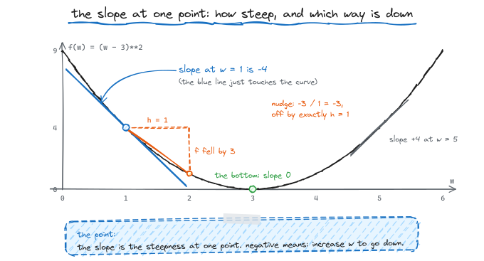
the update rule, and why the minus sign is the whole idea
here is the algorithm:
w = w - lr * slope(w)
lr is the learning rate: a small positive number you choose, such as 0.1. it sets how far each step goes.
why the minus sign? over a short distance, a smooth function changes at the rate its slope says. if you move w by a small amount s, the function changes by about slope * s. gradient descent picks s = -lr * slope. the change is then about
slope * (-lr * slope) = -lr * slope**2
a square is never negative and lr is positive, so this is negative whenever the slope is not zero. the loss goes down. it does not matter whether the slope was positive or negative: the minus sign always turns it into a step toward lower loss.
the word “about” is doing real work. “change = slope * step” is only exact for straight lines. for (w - 3)**2 the exact change is easy to write out. with g for the slope 2(w - 3) and a step s = -lr * g:
f(w + s) - f(w) = g * s + s**2 = -lr * g**2 + lr**2 * g**2 = -lr * g**2 * (1 - lr)
the first part is the downhill promise. the second part, s**2, is the price of the function curving upward under you, and it grows with the square of the step. for small lr the promise wins. at lr = 1 they cancel exactly and the loss does not change at all. above 1 the price wins and the loss goes up. hold on to that boundary; the next sections measure it.
watching it walk
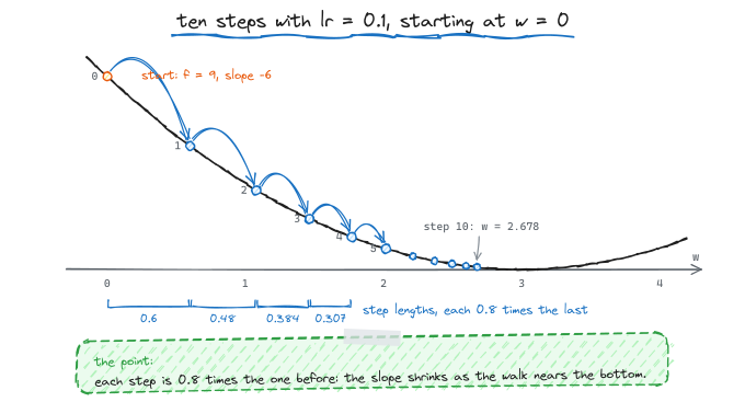
start at w = 0, use lr = 0.1, and print a few steps:
descend.py
# gradient descent on f(w) = (w - 3)**2, whose slope is 2 * (w - 3).
def slope(w):
    return 2 * (w - 3)

def descend(w, lr, steps):
    path = [w]
    for _ in range(steps):
        w = w - lr * slope(w)
        path.append(w)
    return path

path = descend(w=0.0, lr=0.1, steps=50)
for t in [0, 1, 2, 3, 4, 5, 10, 20, 50]:
    w = path[t]
    print(f"step {t:2d}   w = {w:.6f}   f(w) = {(w - 3) ** 2:.6f}   slope = {slope(w):+.6f}")
output of descend.py, pasted unchanged
step  0   w = 0.000000   f(w) = 9.000000   slope = -6.000000
step  1   w = 0.600000   f(w) = 5.760000   slope = -4.800000
step  2   w = 1.080000   f(w) = 3.686400   slope = -3.840000
step  3   w = 1.464000   f(w) = 2.359296   slope = -3.072000
step  4   w = 1.771200   f(w) = 1.509949   slope = -2.457600
step  5   w = 2.016960   f(w) = 0.966368   slope = -1.966080
step 10   w = 2.677877   f(w) = 0.103763   slope = -0.644245
step 20   w = 2.965412   f(w) = 0.001196   slope = -0.069175
step 50   w = 2.999957   f(w) = 0.000000   slope = -0.000086
look at the slope column. each step multiplies it by 0.8: -6, -4.8, -3.84, -3.072. that is not a coincidence. the distance to the answer, w - 3, also shrinks by exactly 0.8 every step, because
new w - 3 = (w - 3) - 0.1 * 2(w - 3) = (1 - 0.2)(w - 3) = 0.8 * (w - 3)
so the steps are big when the slope is steep and small when it is gentle, with no extra code. near the bottom the slope is close to zero, so lr * slope is close to zero, and the walk slows to a crawl. at the exact bottom the slope is zero and w stops moving. that is also how gradient descent “knows” it is done: it does not know. you stop it when the steps or the loss stop changing.
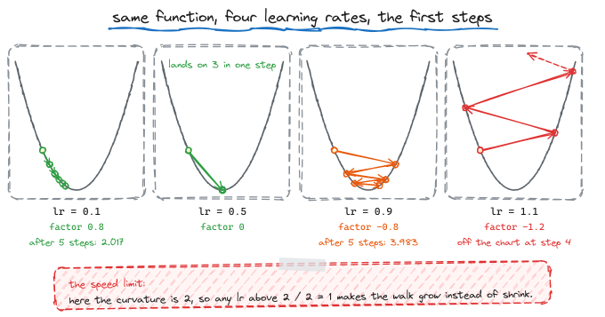
the learning rate is a speed limit set by curvature
run the same thing with six learning rates:
rates.py
# the same descent with different learning rates. |w - 3| is the distance to the answer.
def slope(w):
    return 2 * (w - 3)

print(f"{'lr':<6}{'w after steps 1, 2, 3, 4, 5':<45}{'|w - 3| after 50':>16}")
for lr in [0.01, 0.1, 0.5, 0.9, 1.0, 1.1]:
    w, ws = 0.0, []
    for t in range(50):
        w = w - lr * slope(w)
        ws.append(w)
    first = "".join(f"{x:9.3f}" for x in ws[:5])
    print(f"{lr:<6}{first}{abs(ws[-1] - 3):16.2e}")
output of rates.py, pasted unchanged
lr    w after steps 1, 2, 3, 4, 5                  |w - 3| after 50
0.01      0.060    0.119    0.176    0.233    0.288        1.09e+00
0.1       0.600    1.080    1.464    1.771    2.017        4.28e-05
0.5       3.000    3.000    3.000    3.000    3.000        0.00e+00
0.9       5.400    1.080    4.536    1.771    3.983        4.28e-05
1.0       6.000    0.000    6.000    0.000    6.000        3.00e+00
1.1       6.600   -1.320    8.184   -3.221   10.465        2.73e+04
six different behaviors from one line of code. the formula from the last section explains every row. for this function, each step multiplies the distance to 3 by (1 - 2 * lr):
| lr | factor 1 - 2 * lr |
what happens |
|---|---|---|
| 0.01 | 0.98 | creeps toward 3; still 1.09 away after 50 steps |
| 0.1 | 0.8 | smooth approach |
| 0.5 | 0 | lands exactly on 3 in one step |
| 0.9 | -0.8 | jumps past 3 every step, but each jump is shorter |
| 1.0 | -1 | bounces between 0 and 6 forever |
| 1.1 | -1.2 | each jump is 20% longer than the last; 27,300 away after 50 steps |
two rows deserve a second look. lr = 0.1 and lr = 0.9 end at exactly the same distance, 4.28e-05, because 0.8 and -0.8 shrink the distance equally fast; one approaches from one side, the other zigzags. and lr = 0.5 is perfect for this function, which is the first hint that the right learning rate depends on the function, not on taste.
now make it general. any bowl-shaped function of one weight can be written near its bottom as f(w) = (a / 2) * (w - c)**2. here c is where the bottom is and a is the curvature: how fast the slope itself changes as w moves. (the slope is a * (w - c), so a is the slope of the slope. calculus calls it the second derivative.) for (w - 3)**2, a = 2.
one step multiplies the distance to c by (1 - lr * a). the walk shrinks toward the bottom only if that factor is between -1 and 1, which means
0 < lr < 2 / a
that is the entire stability theory of gradient descent on one weight. the learning rate limit is not a constant like 0.01. it is two divided by the curvature. a sharply curved bowl needs small steps; a flat one allows big ones. the fastest choice is lr = 1 / a, which lands on the bottom in one step, and that is the lr = 0.5 row above.
real losses are not perfect bowls, but a smooth function looks like one near any minimum where it curves upward, with a equal to its curvature there. so the rule holds locally: wherever you are, steps bigger than 2 / curvature make things worse. keep that in mind for the end of the post, where the curvature moves while you train.
many weights: the gradient
real models have many weights, w1, w2, w3, .... the idea carries over with one change: you measure one slope per weight.
the slope of the loss with respect to w1 is computed while holding every other weight fixed: how much does the loss change per unit of w1 alone? same for w2, and so on. calculus calls each of these a partial derivative. the list of all of them is the gradient. the update is the same line, applied to every weight at the same moment:
w1 = w1 - lr * slope_w1
w2 = w2 - lr * slope_w2
...
why is this the right direction to move? suppose you step a small distance in some direction, moving w1 by d1, w2 by d2, and so on. each weight contributes its own slope times its own move, so the loss changes by about
slope_w1 * d1 + slope_w2 * d2 + ...
if you fix how long the step is and ask which direction makes this sum most negative, the answer is: point (d1, d2, ...) exactly opposite to (slope_w1, slope_w2, ...). (this is the cauchy-schwarz inequality: a sum of products like this is most negative when the two lists point in opposite directions.) so the negative gradient is the steepest downhill direction from where you stand.
two consequences matter later. first, “steepest from where you stand” is not “straight at the bottom”. second, if you step along a direction where the loss does not change (along a contour line on a map of the loss), the sum above is zero. so the gradient is always at right angles to the contour lines. on a round bowl that points at the center. on a stretched bowl it does not, and that is the subject of two sections from now.
fitting a line, for real
here is a complete training run of an actual model. the data are ten points near the line y = 2x + 1, with random noise added. the model predicts prediction = m * x + b, so it has two weights, m and b. the loss is the mean squared error: the average over all points of (prediction - y)**2.
the slopes come from one rule of calculus, the chain rule: if the loss depends on the error e, and e depends on m, then the slope of the loss with respect to m is (slope of loss with respect to e) times (slope of e with respect to m). for one point, the loss is e**2 with e = m * x + b - y. the slope of e**2 with respect to e is 2e. the slope of e with respect to m is x, because increasing m by one raises the prediction by x. the slope of e with respect to b is 1. average over the points:
slope for m = average of 2 * e * x
slope for b = average of 2 * e
fit_line.py
# fit prediction = m*x + b to data by gradient descent on the mean squared error.
import random

random.seed(0)
xs = [i / 2 for i in range(10)]                               # 0.0, 0.5, ..., 4.5
ys = [2 * x + 1 + random.uniform(-0.5, 0.5) for x in xs]      # a noisy line y = 2x + 1

def loss(m, b):
    return sum((m * x + b - y) ** 2 for x, y in zip(xs, ys)) / len(xs)

def grad(m, b):
    n = len(xs)
    errs = [m * x + b - y for x, y in zip(xs, ys)]
    dm = sum(2 * e * x for e, x in zip(errs, xs)) / n
    db = sum(2 * e for e in errs) / n
    return dm, db

m, b, lr = 0.0, 0.0, 0.05
for step in range(2001):
    if step in (0, 1, 2, 5, 10, 50, 100, 500, 1000, 2000):
        print(f"step {step:4d}   m = {m:.5f}   b = {b:.5f}   loss = {loss(m, b):.6f}")
    dm, db = grad(m, b)
    m, b = m - lr * dm, b - lr * db

# the exact answer, from the textbook least-squares formula, to compare against
n = len(xs)
mx, my = sum(xs) / n, sum(ys) / n
m_exact = sum((x - mx) * (y - my) for x, y in zip(xs, ys)) / sum((x - mx) ** 2 for x in xs)
b_exact = my - m_exact * mx
L_exact = loss(m_exact, b_exact)
print(f"exact          m = {m_exact:.5f}   b = {b_exact:.5f}   loss = {L_exact:.6f}")
output of fit_line.py, pasted unchanged
step    0   m = 0.00000   b = 0.00000   loss = 38.574544
step    1   m = 1.64917   b = 0.55345   loss = 1.844896
step    2   m = 1.99878   b = 0.68049   loss = 0.164427
step    5   m = 2.08342   b = 0.74358   loss = 0.076704
step   10   m = 2.06867   b = 0.79172   loss = 0.066679
step   50   m = 1.99644   b = 1.01204   loss = 0.037702
step  100   m = 1.96843   b = 1.09749   loss = 0.034053
step  500   m = 1.95834   b = 1.12825   loss = 0.033778
step 1000   m = 1.95834   b = 1.12825   loss = 0.033778
step 2000   m = 1.95834   b = 1.12825   loss = 0.033778
exact          m = 1.95834   b = 1.12825   loss = 0.033778
gradient descent and the textbook formula agree to every printed digit. (they do not land on exactly m = 2, b = 1 because the noise moved the best line; the last row is the best possible line for this data.)
the loss tells a second story. it falls from 38.6 to 0.16 in two steps, then needs about another 100 steps to crawl from 0.077 down to its floor of 0.0338. a fast start followed by a long slow tail is the normal shape of a training curve, and the next section explains where the tail comes from.
stretched bowls: why gradient descent is slow
take the simplest loss with two weights that shows the problem:
f(x, y) = (x**2 + k * y**2) / 2
its slope in x is x and its slope in y is k * y. so it is a bowl with curvature 1 in the x direction and curvature k in the y direction. each direction behaves like its own one-weight problem: x shrinks by (1 - lr) each step and y shrinks by (1 - lr * k).
now the trouble. one learning rate must serve both directions. the steep y direction needs lr < 2 / k, or it explodes. but with lr that small, x shrinks by 1 - lr, which is at best about 1 - 2 / k per step. when k is 1,000, x creeps toward the answer by a fraction of a percent per step.
count the steps, from the point (1, 1) until the distance to the bottom is below one millionth:
bowls.py
# steps needed on a stretched bowl f(x, y) = (x**2 + k * y**2) / 2.
# the slope in x is x, the slope in y is k*y. k is how much steeper one direction is.
import math

def gd_steps(k, lr, tol=1e-6, limit=10**7):
    x, y = 1.0, 1.0
    for t in range(limit):
        if math.hypot(x, y) < tol:
            return t
        x, y = x - lr * x, y - lr * k * y
    return None

def momentum_steps(k, lr, beta, tol=1e-6, limit=10**7):
    x, y, vx, vy = 1.0, 1.0, 0.0, 0.0
    for t in range(limit):
        if math.hypot(x, y) < tol:
            return t
        vx, vy = beta * vx + x, beta * vy + k * y        # velocity: running sum of slopes
        x, y = x - lr * vx, y - lr * vy
    return None

print(f"{'k':>6} {'lr = 1/k':>10} {'best lr':>9} {'momentum':>9}")
for k in [1, 10, 100, 1000, 10000]:
    best = 2 / (1 + k)                                    # best single learning rate (see text)
    s = math.sqrt(k)
    m_lr, m_beta = 4 / (1 + s) ** 2, ((s - 1) / (s + 1)) ** 2   # best momentum settings
    row = [gd_steps(k, 1 / k), gd_steps(k, best), momentum_steps(k, m_lr, m_beta)]
    print(f"{k:>6} {row[0]:>10} {row[1]:>9} {row[2]:>9}")
output of bowls.py, pasted unchanged
     k   lr = 1/k   best lr  momentum
     1          1         1         1
    10        132        71        27
   100       1375       709        95
  1000      13809      7082       321
 10000     138149     70811      1074
the “lr = 1/k” column is the obvious choice: the largest round step that keeps the steep direction safe. the “best lr” column uses lr = 2 / (1 + k), which makes both directions shrink at the same rate (k - 1) / (k + 1); no single learning rate does better on this bowl. even so, the step count grows in direct proportion to k: ten times more stretch, ten times more steps. the ratio of the largest curvature to the smallest is called the condition number, and for gradient descent it is the number that sets the cost of training.
the picture shows what goes wrong. the gradient is at right angles to the contour lines, and on a stretched bowl those lines are long thin ovals, so the gradient points mostly across the valley instead of along it. the walk zigzags from wall to wall and makes slow progress down the length.
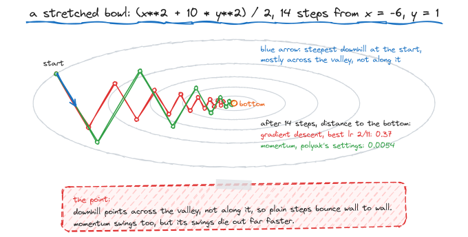
our line fit has this problem too, mildly. a loss with two weights is a bowl with two curvatures along two directions at right angles. for the mean squared error of a line fit they come from a small table of averages, the matrix of second slopes:
excerpt from scaling.py (copied out of the file by script)
def curvatures(xs):
    # the bowl's two curvatures: eigenvalues of [[2*mean(x*x), 2*mean(x)], [2*mean(x), 2]]
    n = len(xs)
    a, c, d = 2 * sum(x * x for x in xs) / n, 2 * sum(xs) / n, 2.0
    mid, r = (a + d) / 2, math.sqrt(((a - d) / 2) ** 2 + c * c)
    return mid + r, mid - r
for the ten points above, x runs from 0 to 4.5 and the two curvatures are about 15.7 and 0.52, a condition number of 30. with lr = 0.05, the distance to the answer along the flat direction shrinks by 1 - 0.05 * 0.52 = 0.974 per step: about 87 steps for every factor of ten. the extra loss above the floor goes with the square of that distance, so it shrinks by a factor of ten about every 43 steps. that is the slow tail in the last section’s output.
the cheap fix: rescale the inputs
now make the inputs bigger. same kind of line fit, but x runs from 100 to 145, like house sizes in square metres. nothing about the problem got harder for a human. watch what it does to gradient descent:
output of scaling.py, pasted unchanged (takes about 30 seconds)
raw x           curvatures   30427.0  0.0271  ratio   1122183  lr 6.57e-05  steps 8082673
standardized x  curvatures       2.0  2.0000  ratio         1  lr 0.5  steps 1
raw x, lr = 2.01 / hi: diverged
eight million steps. two things went wrong at once. squaring numbers in the hundreds makes the curvature for m about 30,000, so the learning rate must be tiny. and because every x is far from zero, m and b are tangled: raise m by 0.01 and every prediction rises by 1 to 1.45, which b has to undo. the bowl is stretched along a diagonal, with a condition number of 1.1 million. go just past the speed limit (lr = 2.01 / largest curvature) and the fit explodes.
the fix is one line before training. standardize x: subtract its average and divide by its spread (standard deviation), so the new inputs have average 0 and spread 1. then the matrix of second slopes is exactly [[2, 0], [0, 2]]: both curvatures are 2, the condition number is 1, and the bowl is perfectly round. gradient descent with lr = 1 / 2 lands on the answer in one step.
eight million steps to one, from centering and rescaling one input. (both parts matter: rescaling alone, or centering alone, still leaves a condition number in the hundreds.) this is why every serious training pipeline normalizes its inputs, and why networks normalize inside their layers too.
momentum: let the steps add up
you cannot always rescale your way out. inside a neural network the stretch comes from the weights themselves, so a second fix works on the steps instead.
look at the zigzag again. across the valley, the slope flips sign every step: up the left wall, up the right wall. along the valley, the slope points the same way every step, just weakly. momentum keeps a running total of past slopes, called the velocity, and steps along that instead of the current slope:
v = beta * v + slope
w = w - lr * v
beta is a number between 0 and 1, usually 0.9. the flipping slopes across the valley mostly cancel inside v. the steady slope along the valley adds up: with beta = 0.9, a slope that keeps pointing the same way builds a velocity up to 1 / (1 - 0.9) = 10 times its size. so momentum takes long steps in the direction that keeps agreeing with itself and short ones in the direction that keeps changing its mind. boris polyak analyzed this method in 1964; it is often called the heavy ball method.
the last column of the bowl table used polyak’s best settings for each k. gradient descent needed steps in proportion to k. momentum needs them in proportion to roughly the square root of k: at k = 10,000 that is 1,074 steps instead of 70,811. those best settings need the two curvatures, which you rarely know, which is why practice settles for beta = 0.9 and a tuned learning rate. the adam section below measures momentum with exactly that.
minibatches: stochastic gradient descent
so far every step used every data point. with a million examples, one step means a million slope calculations. that is where the stochastic version comes in.
the loss is an average over examples, so its slope is the average of the per-example slopes. stochastic gradient descent (sgd) estimates that average from a small random sample, called a minibatch, at every step. the estimate is noisy, but it is right on average: no direction is favored. and it costs batch size slope calculations instead of n.
to compare fairly, give every method the same budget: the total number of single-example slopes it may compute. here are 10,000 points from the line y = 2x + 1 with noise, and the core of the experiment:
excerpt from sgd.py (copied out of the file by script)
def grad(m, b, batch):
    dm = db = 0.0
    for x, y in batch:
        e = m * x + b - y
        dm += 2 * e * x
        db += 2 * e
    return dm / len(batch), db / len(batch)

def run(batch_size, lr, budget, decay=False, checkpoints=(), seed=0):
    rng = random.Random(seed)
    m = b = 0.0
    used, out, step = 0, {}, 0
    while used < budget:
        batch = data if batch_size == N else rng.sample(data, batch_size)
        step_lr = lr / (1 + step / 1000) if decay else lr
        dm, db = grad(m, b, batch)
        m, b = m - step_lr * dm, b - step_lr * db
        used += batch_size
        step += 1
        if used in checkpoints:
            out[used] = loss(m, b)
    return out
output of sgd.py, pasted unchanged
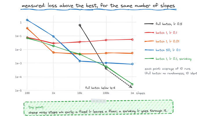
lowest possible loss 0.337407. loss above it after this many single-example slopes
(each number is the average of 10 runs with different random batches):
method                                  100      1,000     10,000    100,000  1,000,000
full batch (10,000), lr 0.5               -          -   0.594776   0.000412   0.000000
batch 50, lr 0.1                   1.426592   0.089946   0.001412   0.001015   0.000857
batch 1, lr 0.1                    0.075513   0.028772   0.035255   0.049442   0.052706
batch 1, lr 0.01                   0.363703   0.005993   0.004774   0.005265   0.005478
batch 1, lr 0.1 shrinking          0.068515   0.018113   0.004358   0.000568   0.000028
three facts sit in this table.
cheap noisy steps win early. after 10,000 slopes, full-batch gradient descent has taken exactly one step and is 0.59 above the best loss. batch-1 sgd with lr = 0.01 has taken 10,000 steps and is at 0.0048, more than 100 times closer. each of its steps is worse; it gets 10,000 times as many.
with a fixed learning rate, sgd never settles. batch 1 at lr = 0.1 stalls around 0.05 above the best and stays there. the weights are not converging to a point; they jitter in a small cloud around it, because every step follows a slightly wrong slope. the size of the cloud follows the step size and the noise: cut lr by 10 and the stall level drops from about 0.05 to about 0.0055. use batches of 50 instead of 1, which divides the noise in the slope estimate by 50 in variance, and the stall level at lr = 0.1 drops by 50 to 60 times, to 0.00086. the rule of thumb that falls out, stall level proportional to lr / batch size, is what these numbers show for this problem.
shrinking the learning rate removes the floor. the last row starts at lr = 0.1 and divides it by 1 + step / 1000, so it takes big steps early and ever smaller ones later. it reaches 0.000028, below every fixed-rate sgd row. herbert robbins and sutton monro proved in 1951 that schedules like this one (the step sizes add up to infinity, but their squares add up to a finite number) converge despite the noise. every decaying learning rate schedule in modern training is a practical answer to this row.
adam: a separate step size for every weight
inside a network you cannot standardize every weight by hand. adam does part of that job automatically: it rescales each weight’s steps, one weight at a time, at every step. diederik kingma and jimmy ba published it in 2014, and it (or its close variant adamw) is the usual default for training networks today.
excerpt from adam.py (copied out of the file by script)
def momentum(lr, beta=0.9):
    def update(w, g, state, t):
        v = state.setdefault("v", [0.0, 0.0])
        for i in range(2):
            v[i] = beta * v[i] + g[i]
            w[i] -= lr * v[i]
    return update

def adam(lr, b1=0.9, b2=0.999, eps=1e-8):
    def update(w, g, state, t):
        m = state.setdefault("m", [0.0, 0.0])
        v = state.setdefault("v", [0.0, 0.0])
        for i in range(2):
            m[i] = b1 * m[i] + (1 - b1) * g[i]           # running average of the slope
            v[i] = b2 * v[i] + (1 - b2) * g[i] ** 2      # running average of the squared slope
            m_hat = m[i] / (1 - b1 ** t)                 # undo the pull toward the zero start
            v_hat = v[i] / (1 - b2 ** t)
            w[i] -= lr * m_hat / (math.sqrt(v_hat) + eps)
    return update
for each weight adam keeps two running averages: m, the average of recent slopes (this is momentum), and v, the average of recent squared slopes. the step is m divided by the square root of v. that division is the whole idea. if a weight’s slopes are always around 1,000, m is about 1,000 and the square root of v is about 1,000, so the step is about lr. if another weight’s slopes are around 0.001, its step is also about lr. the size of the slope cancels out. each weight effectively gets its own learning rate, scaled to undo the size of its own slopes. note what that is not: adam never measures curvature. it only measures how big the slopes have been.
the m_hat and v_hat lines fix a startup problem. both averages start at zero, so after one step m = 0.1 * slope, which is ten times too small. dividing by 1 - 0.9^t undoes this: at t = 1 that divides by 0.1. after the correction the very first step is lr * slope / |slope|, which moves every weight by almost exactly lr, whatever its slope (the tiny eps keeps it from being exact). the defaults above (b1 = 0.9, b2 = 0.999, eps = 1e-8) are the ones from the paper.
now test it against two kinds of stretch, each with 200 data points and two weights. in problem a the two inputs have very different scales: one spans -1 to 1, the other -100 to 100. that stretches the bowl along the weight axes. in problem b both inputs span -1 to 1 but almost always move together, so only their sum is well determined. that stretches the bowl along a diagonal. each method tried 25 learning rates, from 10 down to 0.00001 (each about 1.8 times the next), and kept its best. the last row is adam with its momentum turned off, to see which half of adam does the work:
output of adam.py, pasted unchanged (takes about 5 minutes)
method                                       problem a             problem b
gradient descent                    60150 (lr 0.00018)           4029 (lr 1)
momentum (beta 0.9)                  3320 (lr 0.00032)          195 (lr 1.8)
adam                                      116 (lr 0.1)          431 (lr 3.2)
adam without momentum (b1 = 0)          590 (lr 0.018)         3773 (lr 0.1)
on problem a, adam needs 116 steps where gradient descent needs 60,150 and momentum 3,320. (a finer grid of learning rates would shave some steps off each count; it cannot close gaps this large.) that is the per-weight scaling at work, the same kind of fix as dividing an input by its spread. it is not all of standardizing: the house-size bowl was also stretched along a diagonal, by the tangle between m and b, and that is the kind of stretch problem b tests.
on problem b, momentum beats adam, 195 steps to 431. adam divides each weight by its own scale, one weight at a time, and that cannot undo a stretch along a diagonal, because there the problem is how the weights move together, not how big either one is. adam still beats plain gradient descent here, and the last row says why: with its momentum turned off it needs 3,773 steps, barely better than gradient descent’s 4,029. on problem a, turning momentum off costs far less (590 steps against 116), because there the division does most of the work. this is the honest summary of adam: it fixes scale differences between weights very well, and it is not a cure for every kind of stretch.
where the slopes come from: backpropagation
every method so far needs the slope of the loss with respect to every weight. for a line, we wrote two formulas by hand. for a network with a billion weights, we need a procedure. that procedure is backpropagation: the chain rule from the line-fitting section, applied to every step of the computation, starting from the loss and working backward.
here is the smallest network that has the full shape: one input, one hidden unit, one output, four weights. the hidden unit applies tanh, a function that squashes any number into the range -1 to 1. its slope at z is 1 - tanh(z)**2.
chain.py
# one example through the smallest network: one hidden unit. forward, then backward.
import math

x, y = 2.0, 1.0                      # input and the answer we want
w1, b1, w2, b2 = 0.5, -0.5, 1.5, 0.2   # the four weights

# forward: compute each value from the one before it
z = w1 * x + b1                      # 0.5
h = math.tanh(z)                     # squashes z into the range -1..1
p = w2 * h + b2                      # the prediction
L = (p - y) ** 2                     # the loss
print(f"forward:  z = {z:.4f}   h = {h:.4f}   p = {p:.4f}   L = {L:.4f}")

# backward: slope of L with respect to each value, last value first
dL_dp = 2 * (p - y)
dL_dw2 = dL_dp * h                   # p = w2*h + b2, so p moves by h per unit of w2
dL_db2 = dL_dp * 1
dL_dh = dL_dp * w2
dL_dz = dL_dh * (1 - h * h)          # the slope of tanh at z is 1 - tanh(z)**2
dL_dw1 = dL_dz * x
dL_db1 = dL_dz * 1
print(f"backward: dL/dp = {dL_dp:.4f}   dL/dh = {dL_dh:.4f}   dL/dz = {dL_dz:.4f}")
print(f"slopes:   w1 {dL_dw1:+.4f}   b1 {dL_db1:+.4f}   w2 {dL_dw2:+.4f}   b2 {dL_db2:+.4f}")

# check every slope by nudging the weight and re-running the forward pass
def loss(w1, b1, w2, b2):
    return (w2 * math.tanh(w1 * x + b1) + b2 - y) ** 2
eps = 1e-6
base = [w1, b1, w2, b2]
for i, (name, mine) in enumerate(zip(["w1", "b1", "w2", "b2"], [dL_dw1, dL_db1, dL_dw2, dL_db2])):
    up = base.copy(); up[i] += eps
    dn = base.copy(); dn[i] -= eps
    nudged = (loss(*up) - loss(*dn)) / (2 * eps)
    print(f"check {name}: backprop {mine:+.6f}   nudging {nudged:+.6f}")
output of chain.py, pasted unchanged
forward:  z = 0.5000   h = 0.4621   p = 0.8932   L = 0.0114
backward: dL/dp = -0.2136   dL/dh = -0.3205   dL/dz = -0.2520
slopes:   w1 -0.5041   b1 -0.2520   w2 -0.0987   b2 -0.2136
check w1: backprop -0.504070   nudging -0.504070
check b1: backprop -0.252035   nudging -0.252035
check w2: backprop -0.098731   nudging -0.098731
check b2: backprop -0.213649   nudging -0.213649
read the backward pass from top to bottom. the loss is (p - y)**2, so its slope with respect to p is 2(p - y) = -0.2136. the prediction is p = w2 * h + b2, so p moves by w2 per unit of h, and the slope of the loss with respect to h is -0.2136 * 1.5 = -0.3205. then through the tanh: h moves by 1 - h**2 per unit of z, so the slope with respect to z is -0.3205 * (1 - 0.4621**2) = -0.2520. each weight’s slope is the slope of the value it feeds into, times how much that value moves per unit of the weight. every number matches the nudging check to six decimal places.
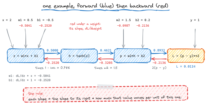
the reason this matters is cost. nudging needs one extra run of the network per weight: a billion runs for one step of a billion-weight model. the backward pass visits each operation once, in reverse, and costs a small constant multiple of one forward pass no matter how many weights there are. that is the only reason training large networks is possible. the method has a long history (seppo linnainmaa described this reverse mode of computing derivatives in 1970), and it became the standard way to train networks after rumelhart, hinton and williams showed in 1986 what it could learn. note what it is and is not: backpropagation computes slopes. gradient descent, or adam, uses them. the two are often confused.
when the curvature moves while you train
put it together: a network with 8 hidden tanh units (25 weights) learns y = sin(x) from 20 points, with backprop for the slopes and plain gradient descent for the steps. the same code runs at two learning rates:
net.py
# a network with one hidden layer of 8 tanh units learns y = sin(x) from 20 points.
# the slopes come from backprop, written out by hand; the weights move by gradient descent.
import math, random

H = 8
xs = [-3 + 6 * i / 19 for i in range(20)]
ys = [math.sin(x) for x in xs]

def train(lr, steps=20000):
    rng = random.Random(0)
    w1 = [rng.uniform(-1, 1) for _ in range(H)]
    b1 = [rng.uniform(-1, 1) for _ in range(H)]
    w2 = [rng.uniform(-1, 1) for _ in range(H)]
    b2 = 0.0

    def forward(x):
        h = [math.tanh(w1[j] * x + b1[j]) for j in range(H)]
        return h, sum(w2[j] * h[j] for j in range(H)) + b2

    history = []
    for step in range(steps + 1):
        n = len(xs)
        L, gw1, gb1, gw2, gb2 = 0.0, [0.0] * H, [0.0] * H, [0.0] * H, 0.0
        for x, y in zip(xs, ys):
            h, p = forward(x)
            L += (p - y) ** 2 / n
            dp = 2 * (p - y) / n                    # slope of the loss for this prediction
            gb2 += dp
            for j in range(H):
                gw2[j] += dp * h[j]
                dz = dp * w2[j] * (1 - h[j] ** 2)   # back through w2, then through tanh
                gw1[j] += dz * x
                gb1[j] += dz
        history.append(L)
        for j in range(H):
            w1[j] -= lr * gw1[j]; b1[j] -= lr * gb1[j]; w2[j] -= lr * gw2[j]
        b2 -= lr * gb2
    worst = max(abs(forward(x)[1] - math.sin(x)) for x in [-3 + 6 * i / 999 for i in range(1000)])
    return history, worst

runs = {lr: train(lr) for lr in (0.05, 0.1)}
print(f"{'step':>6} {'loss, lr 0.05':>14} {'loss, lr 0.1':>14}")
for step in (0, 10, 100, 1000, 2000, 4000, 6000, 7000, 8000, 10000, 20000):
    print(f"{step:>6} {runs[0.05][0][step]:>14.6f} {runs[0.1][0][step]:>14.6f}")
for lr, (hist, worst) in runs.items():
    rises = sum(1 for a, b in zip(hist, hist[1:]) if b > a)
    print(f"lr {lr}: loss rose on {rises} of 20000 steps; worst error on 1000 points: {worst:.4f}")
output of net.py, pasted unchanged
  step  loss, lr 0.05   loss, lr 0.1
     0       0.795893       0.795893
    10       0.053835       0.040949
   100       0.012970       0.009984
  1000       0.006629       0.004689
  2000       0.004660       0.002323
  4000       0.002310       0.002045
  6000       0.000973       0.000371
  7000       0.000575       0.000815
  8000       0.000327       0.000427
 10000       0.000122       0.000201
 20000       0.000034       0.000068
lr 0.05: loss rose on 0 of 20000 steps; worst error on 1000 points: 0.0092
lr 0.1: loss rose on 7350 of 20000 steps; worst error on 1000 points: 0.0155
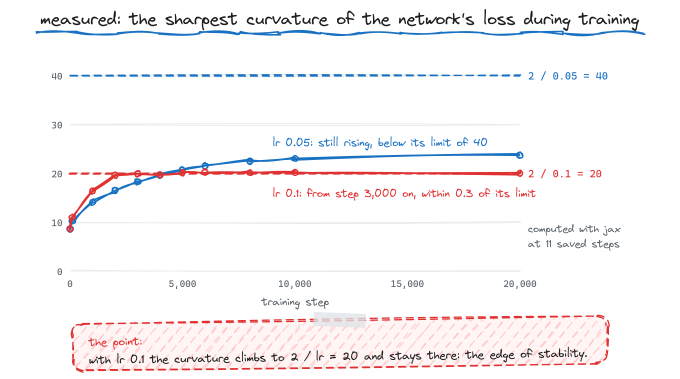
at lr = 0.05 the loss falls on every single step. at lr = 0.1 it rises on 7,350 of the 20,000 steps and ends twice as high. yet lr = 0.1 did not explode either. the stability section says where to look: the curvature. so i measured it: at saved points during both runs, i computed the matrix of second slopes for all 25 weights (with jax, an independent automatic-differentiation library) and took its largest curvature. these are the results:
output of check/sharpness.py, pasted unchanged
sharpest curvature (largest eigenvalue of the matrix of second slopes):
  step   lr 0.05    lr 0.1
     0       8.6       8.6
   100      10.2      11.0
  1000      14.1      16.4
  2000      16.5      19.6
  3000      18.2      19.9
  4000      19.6      19.7
  5000      20.7      20.1
  6000      21.5      20.2
  8000      22.5      20.1
 10000      23.0      20.1
 20000      23.7      20.0
limits 2 / lr: 40 for lr 0.05, 20 for lr 0.1
largest difference, hand backprop vs jax gradient: 8.0e-16
training makes the loss sharper. at lr = 0.05 the largest curvature climbs from 8.6 to 23.7, always below the limit 2 / lr = 40, so every step is stable. at lr = 0.1 it climbs to 20, which is exactly 2 / 0.1, and from about step 3,000 on it stays within 0.3 of 20. the stability section explains the rising loss: wherever the curvature is above 2 / lr, steps along the sharpest direction overshoot. it does not explain why the run recovers. the likely picture is that the overshooting throws the weights to a slightly flatter place, training sharpens them again, and the cycle repeats, so the run lives on the boundary the one-weight formula drew. (eleven snapshots show where the curvature sits, not this mechanism step by step.)
this is not a quirk of a toy. jeremy cohen and coauthors found in 2021 that full-batch gradient descent on neural networks typically behaves this way: the sharpest curvature rises until it hovers just above 2 / lr, and the loss keeps decreasing over long stretches while rising and falling over short ones. they called it the edge of stability. why the sharpness stops at the limit instead of blowing past it is still being worked out.
what gradient descent does not promise
gradient descent stops where the slope is zero. on a bowl, that is the bottom. on anything else, it may not be.
wells.py
# a function with two valleys: f(w) = w**4 - 3*w**2 + w. its slope is 4*w**3 - 6*w + 1.
def f(w):
    return w ** 4 - 3 * w ** 2 + w

def slope(w):
    return 4 * w ** 3 - 6 * w + 1

for start in [-2.0, -0.5, 0.0, 0.5, 2.0]:
    w = start
    for _ in range(1000):
        w = w - 0.01 * slope(w)
    print(f"start {start:+.1f}  ->  w = {w:+.4f}   f(w) = {f(w):+.4f}   slope = {slope(w):+.1e}")
output of wells.py, pasted unchanged
start -2.0  ->  w = -1.3008   f(w) = -3.5139   slope = -1.1e-14
start -0.5  ->  w = -1.3008   f(w) = -3.5139   slope = +8.0e-15
start +0.0  ->  w = -1.3008   f(w) = -3.5139   slope = +8.0e-15
start +0.5  ->  w = +1.1309   f(w) = -1.0702   slope = -9.8e-15
start +2.0  ->  w = +1.1309   f(w) = -1.0702   slope = +9.8e-15
this function has two valleys. start left of about 0.17 and you reach the deep one, at -3.51. start right of it and you reach the shallow one, at -1.07, and stop there for good. at both end points the slope is about 1e-14: both end points have zero slope, and the slope is all gradient descent can see. it never compares one valley with another. start exactly on the hilltop near 0.17, where the slope is also zero, and it never moves at all.
with millions of weights the picture changes in useful ways. points where the slope is zero are mostly saddle points, low in some directions and high in others, and the noise in minibatch slopes tends to push the walk off them. large networks also tend to have many low points of similar quality. that is a description of what usually happens in practice, not a guarantee. on losses that are not bowls, gradient descent finds a place where the slope is zero, and the rest is experience.
how this was checked
every listing above is the file that was run, and every output block is that file’s output, pasted unchanged. excerpts were copied out of the run files by a script, not retyped. the runs used python 3.13 on an intel xeon at 2.10 ghz. all results are step counts and losses rather than timings, and every random number comes from a fixed seed, so the same python version should print the same digits.
a separate test script ran 4,300 randomized checks against independent references (exact formulas, nudging, numpy, jax and optax). most checks call the post’s own functions; checks 1, 2, 6 and 9 re-type the post’s short loops: 1,000 descents against the exact formula c + (w0 - c)(1 - lr * a)^t; 500 checks of the 2 / a stability boundary; 600 line-fit slopes against nudging and 300 against jax automatic differentiation; 200 descents against numpy’s least-squares solver; 300 curvature pairs against numpy’s eigenvalues and 300 matrices of second slopes against jax; 200 stretched-bowl runs against their exact per-direction formula; 200 momentum and adam runs against the optax library’s implementations, step by step for 50 steps; 200 exact best losses against numpy; 300 random networks’ backprop slopes against jax; and 200 two-valley runs against numpy’s roots of the slope. all passed. the network’s hand-written backprop (re-typed from net.py in check/sharpness.py, same seed and same steps) was also compared with jax at 22 saved points of both training runs, agreeing to within 1e-15.
every method in this post is one line of arithmetic away from the next. the skill is knowing which number, the curvature, the noise, or the scale, is the one making your line slow.